This chapter presents some examples of ThingLab in operation. As an introductory example, we will use ThingLab to construct a quadrilateral and view it in several ways. We will then use the system to demonstrate a theorem about quadrilaterals. Before presenting the example, a brief introduction to the ThingLab user interface is needed.

The user interacts with ThingLab via a window, a rectangular area on the computer’s display. The window notion is central to Smalltalk’s user interface philosophy. The ThingLab window described here is typically one of several windows on the screen, with other windows being available for debugging, editing system code, freehand sketching, and so on. [The ThingLab user interface is part of the kernel ThingLab system, and was adapted from the Smalltalk class editor designed by Larry Tesler. See Ingalls 1978, and Goldberg & Robson 1979, for more information about windows and the Smalltalk user interface.]

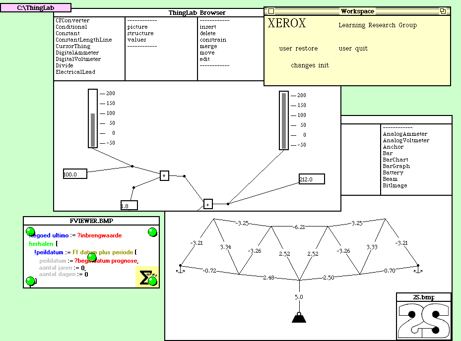
Figure 2.1 - A Smalltalk display

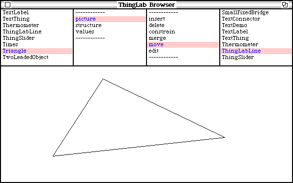
The ThingLab window is divided into five panes: the class pane, the format pane, the messages pane, the arguments pane, and the picture pane. The class pane is a menu of names of classes that may be viewed and edited. Once a class has been selected, a menu of formats in which it can display itself appears in the pane immediately to the right. The class shows itself in the chosen format in the large pane at the bottom of the window labeled picture.

The two remaining panes messages and arguments, contain menus used for graphical editing of the class’s prototype. All editing operations are performed by sending a message to the object being edited; the ThingLab window allows us to compose and send certain kinds of editing messages graphically. The messages pane contains a list of message names, such insert and delete, while the arguments pane contains a list of possible classes for the message argument. The argument itself will be an instance of that class, either newly created or selected from among the parts in the picture. [A black stripe in a menu pane indicates a selected item. Thus in Figure 2.2 Triangle and prototype’s picture have been selected.]

class	format	messages	arguments
pane	pane	pane	pane

picture pane

Figure 2.2 - Panes of the ThingLab window

The first thing we will do in this example is to define the class of quadrilaterals. New classes are always defined as a subclass of some more general class. [If nothing better is available, they can be made subclasses of class Object, the most general class in the system.] We select GeometricObject in the class pane, and the phrase subclass template in the format pane (see Figure 2.3). GeometricObject responds by displaying in the picture pane a template for making a new subclass of itself, which we fill in by typing the name Quadrilateral. The system creates the new subclass. Adds its name to the menu in the class pane, and select the new menu item.

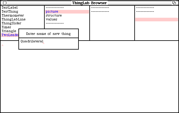
Figure 2.3 - Filling in a subclass template

One of the important features of the ThingLab environment is that the user can define classes by example. More precisely, the structural aspect of a class (its part descriptions and constraints), may be specified incrementally by editing its prototypical instance. We will define the class Quadrilateral in this way. We select the words prototype’s picture in the format pane. The class Quadrilateral creates its prototypical instance, and asks this instance to show itself. So far, the prototype has no parts, and so its picture is blank. In addition to showing its picture, the prototype lists the editing messages that we may sent to it in the message pane, and the possible classes of the arguments for these messages in the argument pane. [The lists of formats, messages, and arguments are each obtained by sending a message to the class being edited. In this case, the lists of formats and messages were both the default inherited form class Object, while the list of argument classes was inherited from GeometricObject.]

We will edit the prototype by adding and connecting four sides. We select the word insert in the message pane, and the word Line in the argument pane. When we move the cursor into the bottom pane, a blinking picture of a line appears, attached to the cursor by one of its endpoints. As the cursor is moved, the entire line follows. When the endpoint attached to the cursor is in the desired location, we press a button. This first endpoint stops moving, and the cursor jumps to the second endpoint. The second endpoint follows the cursor, but this time the first endpoint remains stationary. We press the button again to position the second endpoint (Figure 2.4). [All this behavior arises because the class line declares the two endpoints of each line instance to be attachers.]

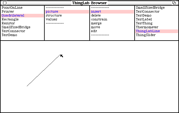
Figure 2.4 - Positioning the second endpoint of a line

We insert another line in the same way. To connect the new line to the first, we position the endpoint attached to the cursor near one of the endpoints of the first line. When the two points are close together, the moving point will lock onto the stationary point, and the line will stop blinking. This indicates that the two points will merge if the button is pressed. We press the button and the points merge. The two lines now share a common endpoint. Also, a record of the merge is kept by the class Quadrilateral. Similarly, we position the other endpoint, and insert the remaining two lines (Figure 2.5).

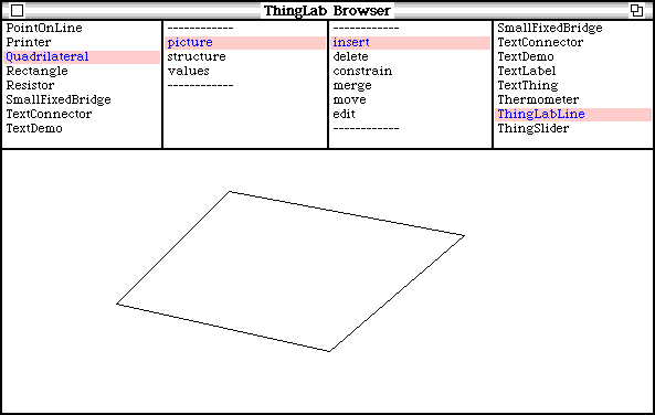
Figure 2.5 - The completed quadrilateral

During this editing session, the system has been updating the structure common to all quadrilaterals that is stored in the class Quadrilateral, as well as saving the particular locations of the prototype’s sides. To see the structure of the class Quadrilateral, we select structure in the menu of formats. The class responds by listing its name, superclasses, part descriptions, and constraints (Figure 2.6) We may also view the values stored in the prototype by selecting prototype’s values (Figure 2.7). [In the table of values, a point with x=10 and y=20 is written as 10¤ 20.]

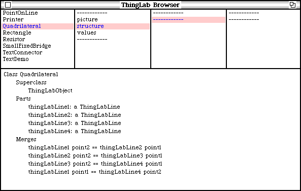
Figure 2.6 - Structure described by the class Quadrilateral

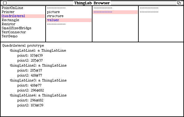
Figure 2.7 - Values of the prototype Quadrilateral

Having constructed the class Quadrilateral, we index it in the list of classes useful in geometric constructions. [This is currently done by typing and executing a Smalltalk statement; eventually this should be handled graphically.]

We may now use the new class in demonstrating a geometry theorem. The theorem states that given an arbitrary quadrilateral, if one bisects each of the sides and draws lines between the adjacent midpoints, the new lines will from a parallelogram. [The idea of demonstrating this theorem with ThingLab was suggested by John Seely Brown.] In the construction, instances of the class MidPointLine will be used to represent bisected lines. The class MidPointLine specifies that each of its instances has two parts: a line and a point. In addition, it has a constraint that, for each instance, the point be halfway between the endpoint of the line. This class has already been constructed by an experienced user as part of the package of geometric classes. Let’s look at it in two different formats (Figures 2.8 and 2.9).

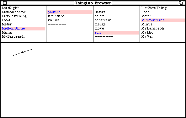
Figure 2.8 - Picture of the prototype MidPointLine

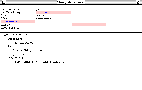
Figure 2.9 - Structure described by the class MidPointLine

To perform the construction, we will make a new class named QTheorem. As before, we create it as a subclass of GeometricObject, and define it by example. We select prototype’s picture in the format pane. We will first add an instance of class Quadrilateral as a part. We select insert and Quadrilateral. As we move the cursor into the bottom pane, a blinking picture appears of a quadrilateral whose shape has been copied from the prototype. Since we didn’t declare otherwise, the entire instance is the attacher. [Another reasonable choice would have been to designate the four corners as attachers. Designation of attachers is currently handled by typing and executing a Smalltalk statement.] We position the quadrilateral and press a button.

The next step is to add midpoints to the sides of the quadrilateral. We select the message constrain and the argument MidPointLine. A blinking picture of an instance of MidPointLine appears. As with the quadrilateral, the shape of the new MidPointLine instance has been copied from the prototype. When the action is constrain, its line part is attacher. We move the MidPointLine near the center of one of the sides of the quadrilateral and press the button, thus merging the line part of the midpoint with the side of the quadrilateral. Similarly, we add midpoints to the other tree sides (Figure 2.10).

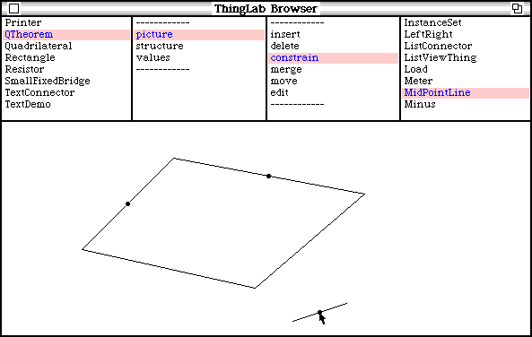
Figure 2.10 - Adding a midpoint

The last step is to add four lines connecting the midpoints to form the parallelogram. If we make a mistake along the way, the delete message may be used to remove the offending object. For example, to delete a line, we select delete and line. A complemented image of a line appears that is attached to the cursor (Figure 2.11). This anti-line sticks to lines in the picture. When the position it near the unwanted line and push the button, the line and the anti-line annihilate each other.

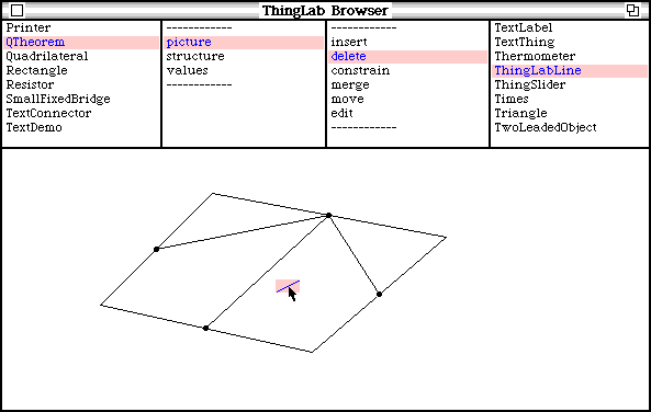
Figure 2.11 - Deleting a line

Once the construction is complete, we may move any of the parts of the prototype QTheorem and observe the results. In general, it will not be enough for the system simply to move the selected part; because of the constraints we have placed on the object, other parts, such as the midpoints may need to be moved as well to keep all the constraints satisfied. Suppose we want to move a vertex. We select the message move and the argument Point. A blinking point appears in the picture that is attached to the cursor. We position it over the vertex to be moved and hold down a button. The vertex follows the cursor until the button is released (Figure 2.12). [The first time we try to move the vertex, there will be a long pause as the system plans how to satisfy the constraints.] We notice that indeed the lines connecting the midpoints form a parallelogram no matter how the quadrilateral is deformed. The theorem remains true even when the quadrilateral is turned inside out!

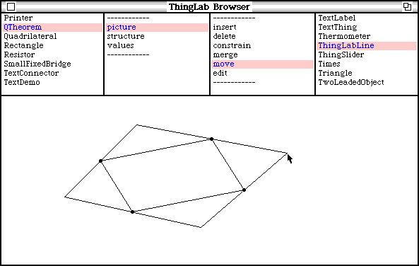
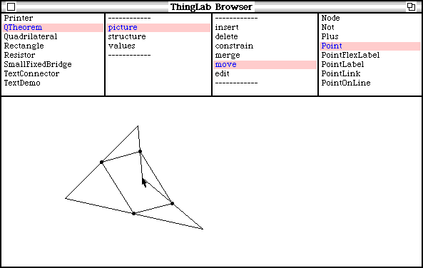
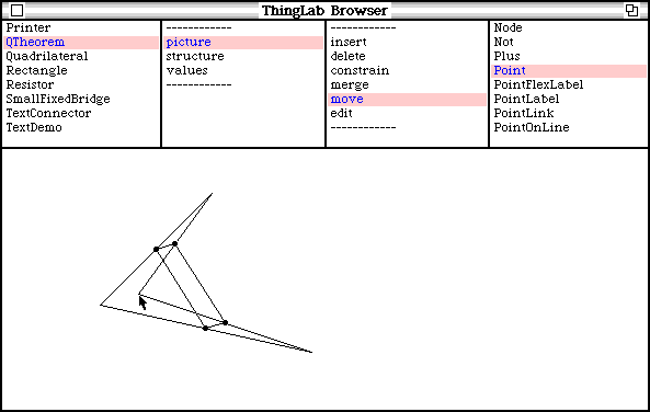
Figure 2.12 - Moving a vertex of the quadrilateral

A few comments about the constraint satisfaction process are now in order. The user described how QTheorem should behave in terms of the midpoint contstraint and the various merges, but not by writing separate methods for moving each part of QTheorem. The midpoint constraint (as defined by an experienced user) describes methods that can be invoked to satisfy itself. Three such methods were specified: the first asks the midpoint to move to halfway between the line’s endpoints; the second asks one of the line endpoints to move; and the third asks the other endpoint to move. It was up to QTheorem to decide which of these methods to invoke, and when and in what order to use them. A number of techniques for doing this have been built into the system, as will be described in Chapter 5.

In general the constraints on an object might specify its behavior incompletely or redundantly, or they might unsatisfiable. QTheorem, for example, is underconstrained. The behavior we observed was only one way of moving the vertex while satisfying the constraints. Two other possibilities would have been for the entire object to move, or for the midpoints to remain fixed while the other vertices moved. Neither of these responses would have been pleasing to us as human observers. [If we had wanted the entire object to move, we would have specified move QTheorem instead.] Therefore, besides the more mathematical techniques for finding some way to satisfying its constraints, or for deciding that they are unsatisfiable, an object can also take the user’s preferences into account in deciding its behavior. In this case, the midpoint constraint specified that the midpoint was to be moved in preference to one of the endpoints of the line.

We might override this information by anchoring the midpoints, as in Figure 2.13. [The anchor symbol indicates a constraint that the anchored point may not be moved during constraint satisfaction.]

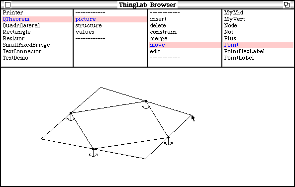
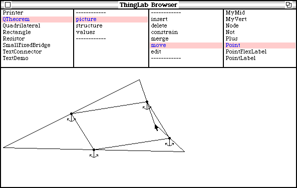
Figure 2.13 - A quadrilateral with anchored midpoints

In this second example, we will construct some graphical programs for a simulated calculator. It is interesting to note that the use of ThingLab for this application was not anticipated – all the classes used here were designed only afther the system has been running for some time. However, there is a strong resemblance between the calculator parts and electrical circuit parts, and ThingLab was designed to be able to simulate simple electrical circuits.

Some useful classes for building calculator programs have already been designed by an experienced user. One simple but important class is NumberNode. An instance of NumberNode has two parts: a real number and a point. Its purpose is to provide a graphical representation of a register in the calculator. Another class is NumberLead consisting of a number node and a attached line. As with leads on electrical components, it is used to connect together parts of the calculator.

Using these building blocks, classes that represent the various arithmetic operations have been defined. First, there is a general class NumberOperator. The parts of a NumberOperator are a frame for displaying the operator’s symbol, and three number leads that terminate on the edges of the frame. The frame and the nodes at the ends of the three number leads are all designated as attachers. Four subclasses of NumberOperator are defined, namely Plus, Minus Times and Divide.

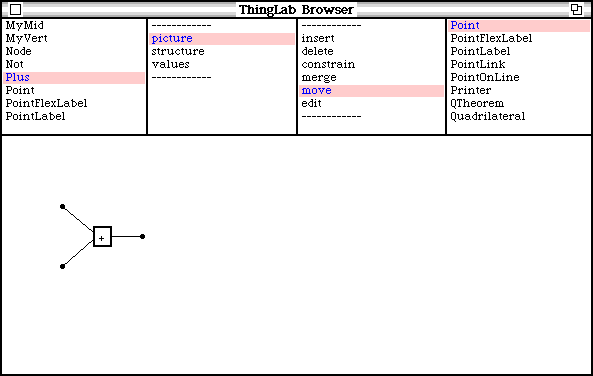
Figure 2.14 - Picture of the prototype for plus

Plus, for example, has three number leads with number nodes at the ends, which are inherited form NumberOperator. It has an added constraint that the number at the node on the right always be the sum of the numbers of the leads on the left. The classes for Minus, Times and Divide prototypes have been defined analogously.

To view and edit a number at a node, the class NumberPrinter has been constructed. Its parts are a number lead and an editable piece of text. Also, it has a constraint that the number at its node correspond to that displayed in the text. If the node’s number changes, the text will be updated; if the text is edited, the node’s number will be changed correspondingly. A special kind of NumberPrinter is a Constant. For constants, the constraint is one way. The text may be edited, thus changing the number; but the number may not be changed to alter the next.

Using these parts, let’s construct a Centigrade to Fahrenheit converter. After creating a new class TemperatureConverter, we choose the prototype’s picture format for viewing and editing it. Next, we select the word insert in the message pane, and the word Times in the tool pane. As we move the cursor into the picture pane, a blinking picture of an instance of the class Times appears. We position the frame that holds the multiplication symbol, and then the three nodes. Following this, we insert a Plus operator in the same manner connecting one of the nodes on its left to the nodes of the times operator on the right. [The author has avoided the terms input and output nodes in describing these operators, since as shall be seen, information flow is not restricted in this way.] Finally, we insert two instances of Constant connecting them to the appropriate nodes of the operators. We then invoke the edit text message, and change the constants to 1.8 and 32.0. The result is shown in Figure 2.15. [Incidentally, note the use of generic editing messages: the same insert message is used to insert lines, arithmetic operators, and resistors; the edit text messages is used both to edit the value of a constant and to edit a paragraph in a document.]

Figure 2.15 - Picture of the completed Centigrade to Fahrenheit Converter

Once the converter has been defined, we may use it as a part of other objects (i.e., as a subroutine). As an example of this, we define a new class PrintingConverter. We add an instance of TemperatureConverter as a part, and also two instances of NumberPrinter to display the Centigrade and Fahrenheit temperatures (Figure 2.16). If we edit the Centigrade temperature, the PrintingConverter will satisfy its constraints by updating the numbers at its nodes, and the Fahrenheit temperature displayed in the frame on the right.

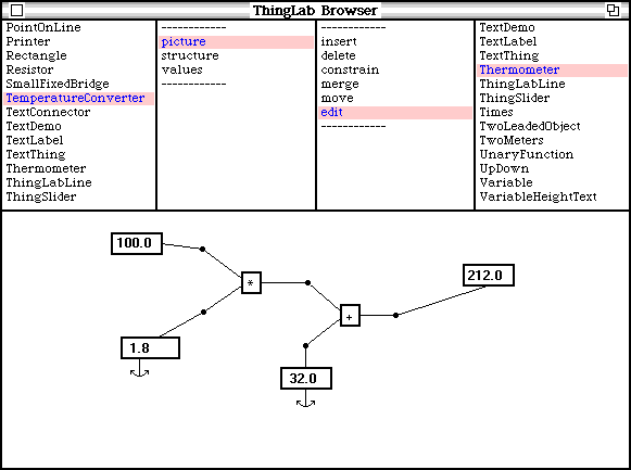
Figure 2.16 - A PrintingConverter

However, because of the multi-way nature of the constraints, the device works backwards as well as forwards! Thus, we can edit the Fahrenheit temperature, and the Centigrade temperature will be updated correspondingly (Figure 2.17). This demonstrates the need for the special class Constant – without it, the system could equally well have satisfied the constraints by changing one of these coefficients rather than the temperatures.

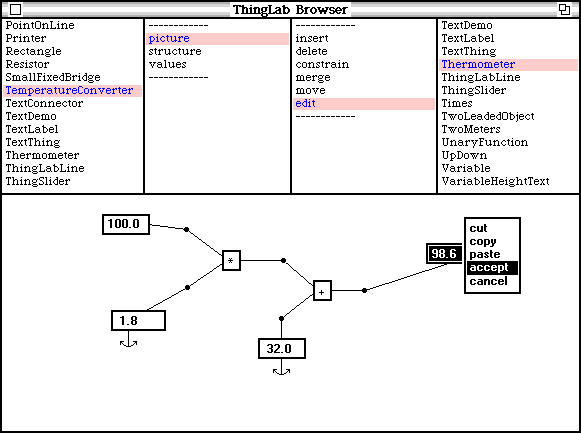
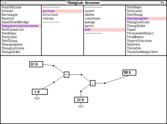
Figures 2.17 - Editing the Fahrenheit temperature

We may also connect the converter to other types of input-output devices, for example, a simulated thermometer. We find an experienced ThingLab user, and ask her to define a Thermometer class for us. A thermometer has a number lead for connecting it with other devices, and a constraint that the height of the mercury be proportional to the number at its node. We then build another class in analogy with PrintingConverter, and again use an instance of TemperatureConverter as one of its parts. This time, however, we hook up the converter to instances of class Thermometer. When the construction is complete, we can select move and point, and grab either of the columns of mercury with the cursor. When we move one of the columns up or down, the other column moves correspondingly (Figure 2.18).

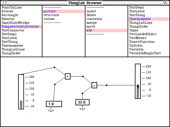
Figure 2.18 - The temperature converter with thermometers for input and output

After experimenting with the converter, we might try building a more complex device, such as the network for solving quadric equations shown in Figure 2.19.

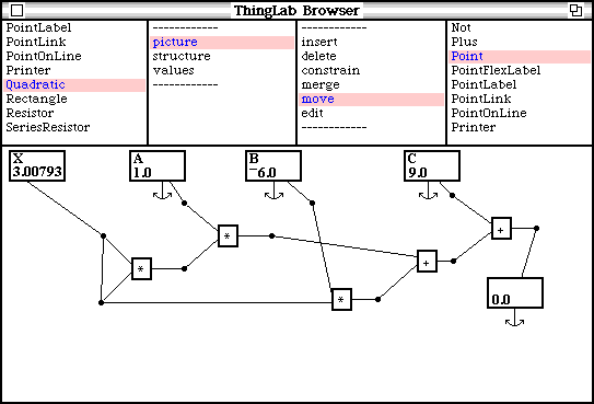
Figure 2.19 - A quadratic equation network

When we edit any of the constants, the value in the frame on the left will change to satisfy the equation. In the picture, the coefficients of the equation X² –6X + 9 = 0 have been entered, and a solution X = 3 has been found. Unlike the temperature converter examples, in this case the system was unable to find a one-pass ordering for solving the constraints, and has resorted to the relaxation method. [Note that the graph structure has loops in it.] Relaxation will converge to one of the two roots of the equation, depending on the initial value of X.

Now let’s try changing the constant c from 9 to 10. This time, the system puts up an error message, protesting that the constraints cannot be satisfied. Some simple algebra reveals that the roots of this new equation are complex – but the number nodes hold real numbers, and so the system was unable to satisfy the constraints.

A better way of finding the roots of a quadratic equation is to use the standard solution to the quadratic equation AX² + BX + C = 0, namely X = (-B ± ( B² – 4AC) ^½ ) / 2A. The system can be told about this canned formula by embodying it as a constraint. We find an expert user, who constructs a class quadraticSolver for us (Figure 2.20). The parts of an instance of QuadraticSolver include four NumberNodes a, b, c, and x, and a constraint that X = (-B + (B² – 4AC) ^½ ) / 2A. [Since the class NumberNode doesn’t allow multiple values, in the QuadraticSolver’s constraint one of the roots has been chosen arbitrarily as the value for X. A more general solution would be to define a class MultipleRoots, and set up the constraint so that it determined both the number of roots and their values.]

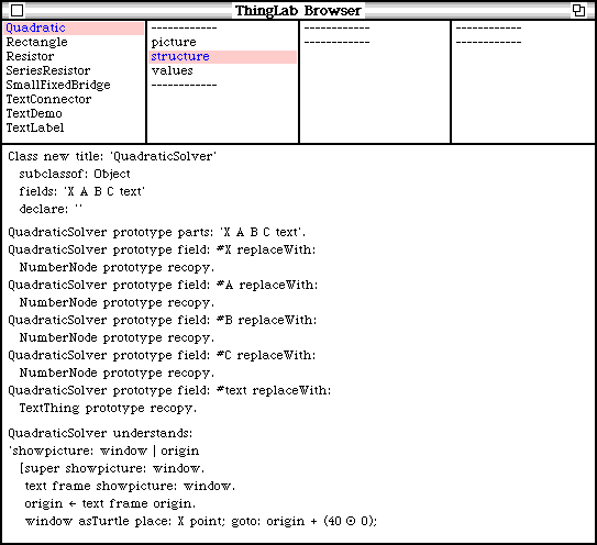
Figure 2.20 - Constructing the class QuadraticSolver

When then insert an instance of QuadraticSolver into the network, merging its number nodes with the appropriate existing nodes in the network (Figure 2.21). Now, the system can find a simple one-pass ordering for satisfying the constraints, and doesn’t need to use relaxation

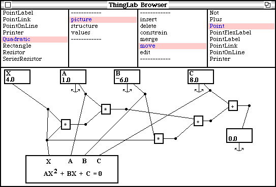
Figure 2.21 - The network after adding an instance of QuadraticSolver

In inserting an instance of QuadraticSolver to the network, we have added another view of the constraints on X. In the sense that the permissible values of X are the same with or without it (ignoring the multiple root problem), the new constraint doesn’t add any new information. However, QuadraticSolver’s constraint is computationally better suited to finding the value of X. This technique of introducing multiple redundant constraints on an object is an important way of dealing with circularity.

Beyond this thesis, one of directions of this research has been toward a complete programming language organized around constraints. Such a language is proposed in Chapter 6. This example gives some interesting glimpses of what such a language might be like. QuadraticSolver could have been described by constructing a network, as with the original class Quadratic, rather than having a specially-defined constraint. However, if one tries sketching the network for QuadraticSolver, one will find that it is not very illuminating, and also takes up much more space than the algebraic form. Even with the original network, the diagram is much harder to understand than the written equation for people who know algebra, It would be nice, therefore, to have a language in which, for example, the algebraic constraint AX² + BX + C = 0 had the same semantics as the diagram.

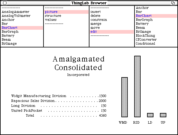
Figure 2.22 - A document with constrains

The example shown in Figure 2.22 demonstrates the use of constraints in describing a dynamic document. The document consists of a number of paragraphs of text, and four instances of BarGraph. Each instance of BarGraph has a constraint that relates the height of the bar to the number displayed in a text field. In addition, the document as a whole has a constraint that the sum of the numbers of employees in each division be equal to the total at the bottom.

We can edit one of the fields containing the number of employees in a division. When we change the number of employees in United PickPocket from 200 to 800 and issue the accept command, the sum will be updated, and the height of the corresponding bar will change appropriately to satisfy all the constraints ( Figure 2.23).

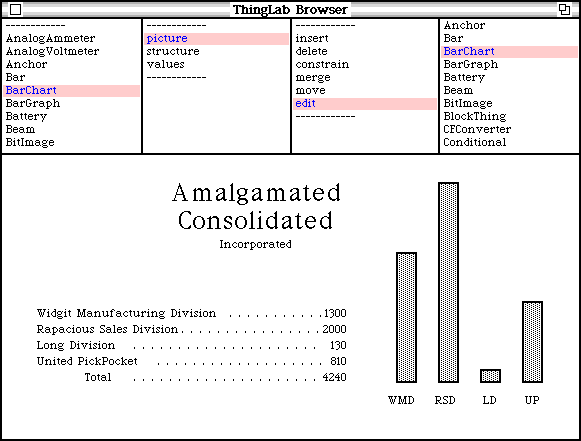
Figure 2.23 - The document after editing the number of employees in United PickPocket

Also, we can pick up the top of one of the bars with the cursor. As we move it up or down, the corresponding number and the total will change (Figure 2.24).

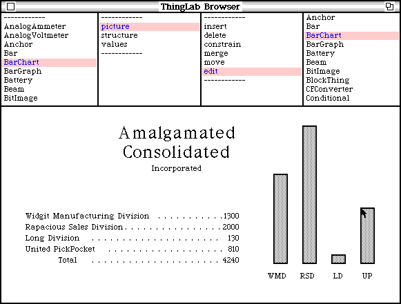
Figure 2.24 - Moving the top of a bar

The previous example demonstrated the use of constraints on the contents of a document; Figure 2.25 shows an example of a constraint on layout.

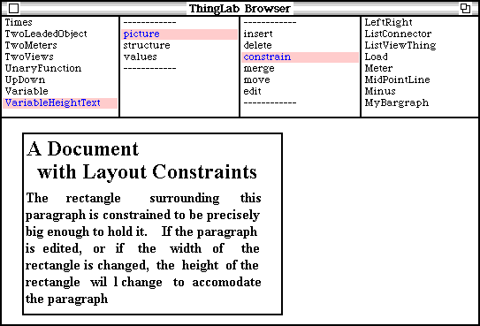
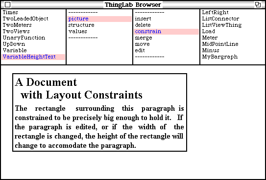
Figure 2.25 - A document with layout constraints

The text object has a constraint that the height of the rectangle be such that the rectangle is precisely big enough to hold the paragraph. If we change the width of the rectangle or edit the paragraph, the rectangle’s height will adjust itself accordingly.

The example in Figure 2.26 illustrates how the shape of a paned window, such as the used in the ThingLab user interface, can be specified by constraints. The basic building block is the class Rectangle. Using Rectangle, an experienced user has defined two new building blocks, namely a class LeftRight and a class UpDown. The parts of an instance of LeftRight are a pair to rectangles constrained to be side-by-side and of the same height; UpDown is defined analogously. Using these classes in turn, instances of LeftRight and UpDown may be connected together by merging the appropriate corners to from a paned window.

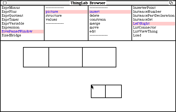
Figure 2.26 - Building a paned window

To change a corner of one of the panes, we may select move point; to move a pane as a unit, we may select move Rectangle. As we move the part, the other parts of the paned window will adjust themselves to satisfy all their constraints (Figure 2.27).

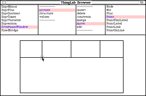
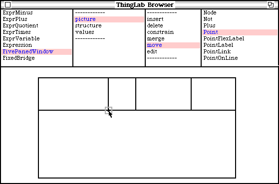
Figure 2.27 - Moving the corner of a pane in a paned window

This example demonstrates some more things that can be done with multiple views in ThingLab. In Figures 2.28 and 2.29, a point in used to represent to an object. Various views can be connected to the object; as the object changes, the views are updated correspondingly.

Figure 2.28

Two views of a triangle

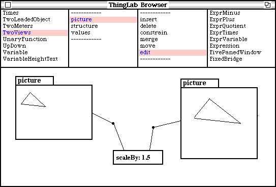
Figure 2.29

Two triangles connected by a scaling constraint

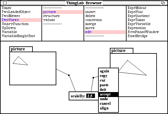
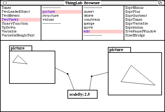
Figure 2.30 - Editing the scaling constraint

In Figure 2.29, two triangles are connected by a constraint that one triangle be 1.5 times as big as the other. If we edit the text in the constraint description, making the scale factor 2.5, the triangle on the right increases in size appropriately.

This example has been taken directly from Sketchpad [Sutherland 1963]. For use in constructing bridge simulations, a class Beam, a class Weight, and a class Anchor have been defined. The beams have a constraint that they obey Hooke’s Law. Using these classes, we can construct a simulation of a bridge. When we apply the weight, the beams extend and compress accordingly (Figure 2.31). In this case the constraint satisfier couldn’t find a one-pass ordering for satisfying these constraints, and so relaxation was used. [Each beam has displayed how much it has lengthened or shortened. A positive number indicates an extension; a negative number indicates a compression.]

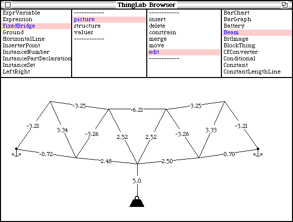
Figure 2.31 - A bridge under load

A simulation of a simple electrical circuit will now be presented. To illustrate a typical set of building blocks for a given domain, the basic classes used in constructing the circuit will be shown. These classes have been defined by an experienced user of the system. Using these classes. a less sophisticated user could then employ them in constructing a simulation such as that shown here.

The building blocks used in the circuit are resistors, batteries, meters, and wires. Also, there are two other kinds of objects used in connecting together the components of the circuits: nodes and leads. A node is a connection point in the circuit; its parts include a voltage and a graphical screen location. A lead is a terminal of one of the components such as a resistor or a meter, and has as its parts a node and a current. To connect, say, two resistors together, the node from the lead of the first resistor is merged with the node from the lead of the second.

            [current ¬ 0.0 – (currents excluding: current) sum]

The parts of a node are a voltage, a set of currents flowing into that node, and a screen location. The constraint is Kirchhoff’s law: it specifies that the sum of the currents into the node be 0. The information under the constraint’s rule is a method for computing any one of the currents, given the values of all the others.

         Voltage ¬ 0.0

A ground is a kind of node whose voltage must be 0.

A lead represents one of the connecting wires of a component.

         Lead1 node current ¬ 0.0 – lead2 node current

         Lead2 node current ¬ 0.0 – lead1 node current

This is an abstract superclass used in defining components with two leads. Its has a constraint that the current flowing out of one lead be equal and opposite to the current flowing out of the other.

         Lead1 node voltage ¬

         Lead2 node voltage ¬

         Lead1 current ¬

         resistance ¬ label text asFloat

         label text ¬ resistance asString asParagraph

In addition to the constraint inherited from TwoLeadedObject, a resistor has an Ohm’s law constraint, and a constraint that its resistance correspond to the text in its label. In the Ohm’s law constraint, resistance has been designated as reference only, so that the system will have to satisfy the constraints by changing the voltages and currents in the circuit, rather than by changing the values of the components

         Lead1 node voltage ¬ lead2 node voltage + internalVoltage

         Lead2 node voltage ¬ lead1 node voltage – internalVoltage

         InternalVoltage ¬ label text asFloat

         Label text ¬ internalvoltage asString asParagraph

         Lead1 node voltage ¬ lead2 node voltage

         Lead2 node voltage ¬ lead1 node voltage

A wire is itself a kind of two leaded object. Its constraint specifies that the wire be a perfect conductor. [If it were important to represent the resistance of a real wire, this could be done using an instance of Resistor instead.]

         Lead1 node voltage ¬ lead2 node voltage

         Lead2 node voltage ¬ lead1 node voltage

         Reading text ¬ lead1 current as text

         Lead1 current ¬ 0.0

         Reading text ¬ (lead1 node voltage – lead2 node voltage) as Text

Both the class Ammeter and the class Voltmeter describe perfect meters. An instance of Ammeter has no voltage drop across it; an instance of Voltmeter draws no current.

The pictures for these building blocks were defined by writing an appropriate Smalltalk method. For example, the picture of a node is a dot if the number of currents in its set is three or more, and otherwise nothing; the picture of a resistor is the usual symbol, along with an editable label indicating its resistance.

Using the components, we may construct a voltage divider (Figure 2.32)

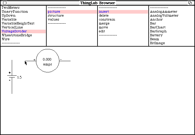
   Figure 2.32 - Building a voltage divider

The nodes at the ends of the leads of the components are designated as attachers by the class TwoLeadedObject. Thus, when inserting the ammeter, the node at the end of each lead will try to merge with an existing node in the circuit.

Figure 2.33 - The completed voltage divider

After the circuit has been completed (Figure 2.33), we may change its parameters and observe the result (Figure 2.34).

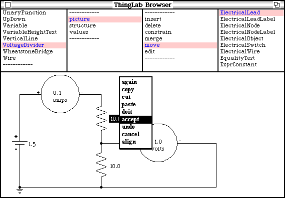
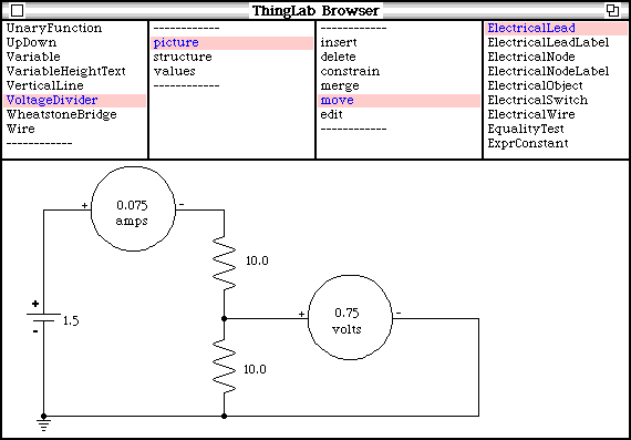
Figure 2.34 - Changing a resistance in the voltage divider

Again, in this case, the system was unable to satisfy the constraints in one pass, and has used relaxation. A discussion of constraint satisfaction for this example, and another example of the use of multiple views to eliminate the need for relaxation, may be found in Chapter 5.